Building a 6TB Data Warehouse From Scratch: Lessons I Wish I Knew Earlier

The first time I ran SELECT pg_database_size('credit_bureau_dw') and saw 6.2 terabytes staring back at me, I had one thought: "This is either going to be the most educational experience of my career or the thing that ends it."

It turned out to be the former, but not without some painful lessons along the way. I spent two years at Credit Bureau Malaysia building and maintaining a PostgreSQL data warehouse that ingested credit data from every major financial institution in the country. Millions of records flowing in daily, regulatory reporting deadlines that could not slip by a single hour, and queries from risk analysts who needed answers in seconds, not minutes.

Here is what I wish someone had told me before I started.

When I joined, the data lived in a patchwork of legacy systems and flat files. The "data warehouse" was a generous term for a collection of SQL Server databases that had grown organically over years. My mandate was to consolidate everything into a proper analytical warehouse.

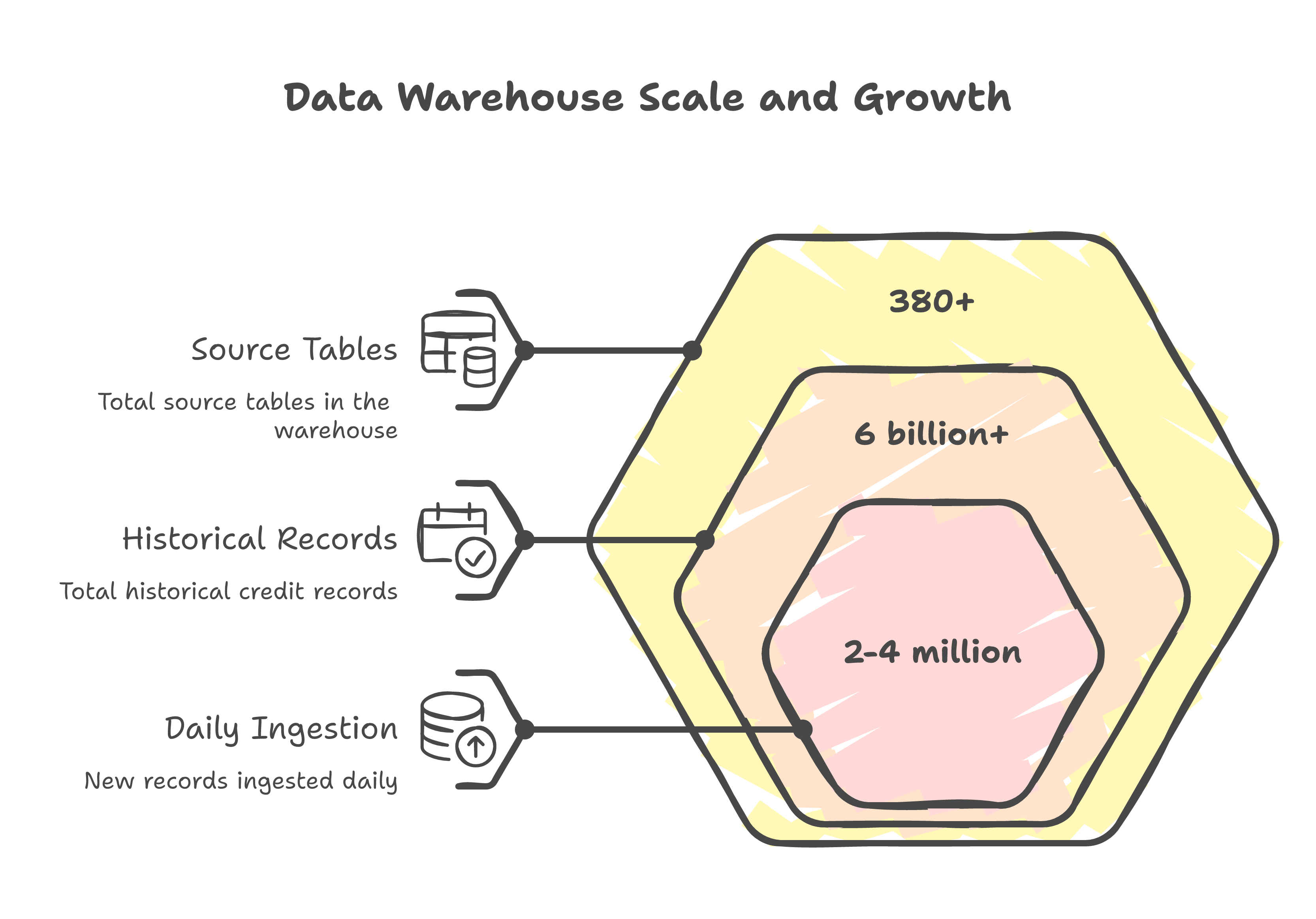
The initial data audit revealed the scope:

• 380+ source tables across multiple source systems
• 6+ billion rows of historical credit records
• Daily ingestion of 2-4 million new records from banking partners
• Regulatory requirement: full historical auditability going back 7 years

I had built data pipelines before. Small ones. The kind where you can SELECT * from your staging table and eyeball the results. This was a different animal entirely.

The single most consequential decision in any data warehouse project is the schema design, because unlike application databases, you cannot easily refactor a warehouse schema once it is loaded with terabytes of historical data.

Star Schema With a Twist

We went with a modified star schema. The core fact tables tracked credit events (applications, disbursements, repayments, defaults), and dimension tables covered entities (borrowers, institutions, products, time).

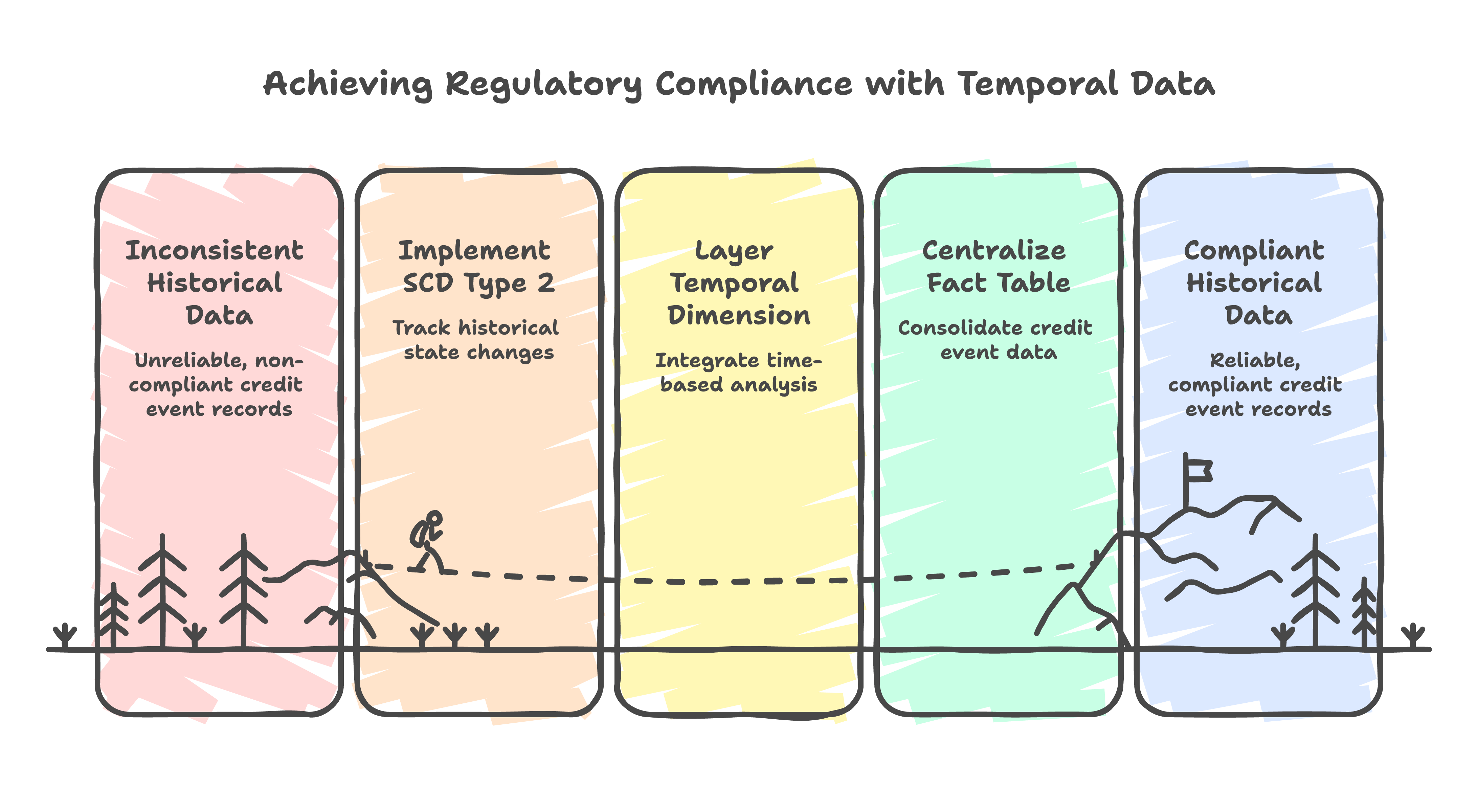
The twist was what I call temporal dimension layering. Credit bureau data has a unique property: the same entity can have different attributes at different points in time, and you need to query both the "as-of" state (what did we know at time T?) and the "current" state (what do we know now?).

CREATE TABLE dim_borrower (
    borrower_key    SERIAL PRIMARY KEY,
    borrower_id     VARCHAR(20) NOT NULL,
    name            VARCHAR(200),
    ic_number_hash  VARCHAR(64),      -- SHA-256 for PII protection
    risk_grade      CHAR(2),
    effective_from  DATE NOT NULL,
    effective_to    DATE DEFAULT '9999-12-31',
    is_current      BOOLEAN DEFAULT TRUE,
    record_source   VARCHAR(50),
    load_timestamp  TIMESTAMP DEFAULT CURRENT_TIMESTAMP
);

CREATE INDEX idx_borrower_current ON dim_borrower (borrower_id)
    WHERE is_current = TRUE;

The effective_from / effective_to pattern (Type 2 Slowly Changing Dimension) was essential. Regulators could ask "what was this borrower's risk grade when the loan was approved in 2019?" and we needed to answer that accurately, not with the current risk grade.

Partitioning Strategy

With 6TB of data, query performance lives or dies on your partitioning strategy. We partitioned fact tables by month using PostgreSQL's native declarative partitioning:

CREATE TABLE fact_credit_events (
    event_id        BIGSERIAL,
    event_date      DATE NOT NULL,
    borrower_key    INTEGER REFERENCES dim_borrower,
    institution_key INTEGER REFERENCES dim_institution,
    event_type      VARCHAR(20),
    amount          NUMERIC(18, 2),
    -- ... additional columns
) PARTITION BY RANGE (event_date);

CREATE TABLE fact_credit_events_2024_01
    PARTITION OF fact_credit_events
    FOR VALUES FROM ('2024-01-01') TO ('2024-02-01');

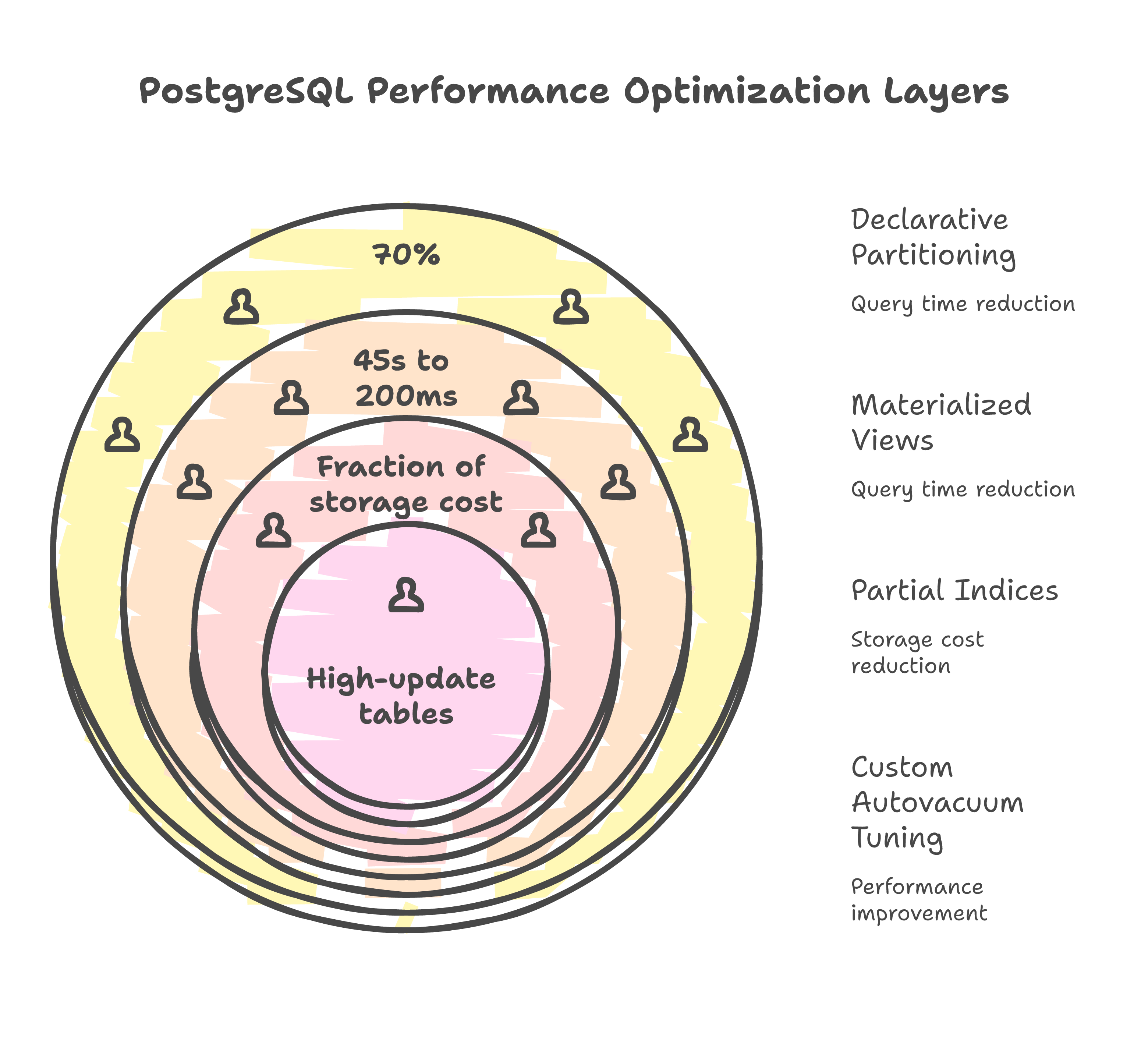
Partitioning cut our average query times by roughly 70% for date-bounded queries, which was the vast majority of analytical workloads. But it introduced operational complexity that I underestimated.

The partition management problem: Every month, you need a new partition. Miss it, and inserts fail. We automated this with a maintenance function that pre-creates partitions 3 months ahead, but the first time it failed silently during a holiday weekend... let's just say I learned the importance of monitoring partition existence as a health check.

The textbook version of ETL is straightforward: extract from sources, transform to match your schema, load into the warehouse. The production version is a minefield.

The Replication Challenge

Our data came from the central bureau's consolidated feeds, covering credit records from multiple financial institutions across the country. The bureau data arrived in varying formats and quality levels that required extensive cleaning and normalization.

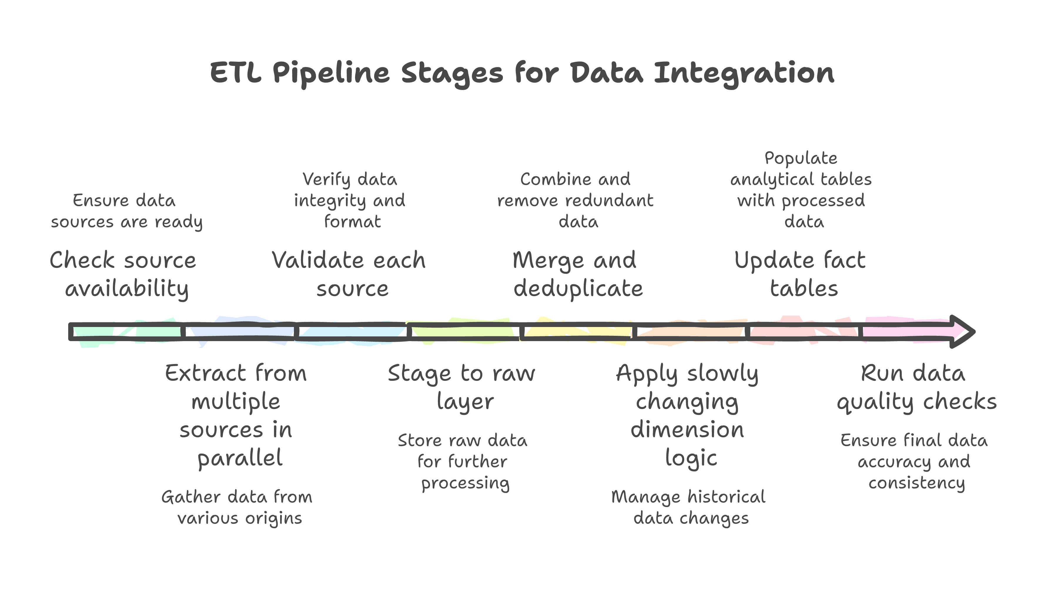
We built the ETL pipeline with Apache Airflow, and the DAG structure reflected the messy reality:

# Simplified DAG structure
with DAG("daily_credit_ingestion", schedule_interval="0 6 * * *") as dag:
    check_sources = check_all_source_availability()

    extract_tasks = []
    for source in INSTITUTION_SOURCES:
        extract = extract_from_source(source)
        validate = validate_source_data(source)
        stage = stage_to_raw_layer(source)

        check_sources >> extract >> validate >> stage
        extract_tasks.append(stage)

    merge_and_deduplicate = merge_staged_data()
    apply_scd = apply_scd_logic()
    update_facts = update_fact_tables()
    run_quality_checks = run_dq_suite()

    extract_tasks >> merge_and_deduplicate >> apply_scd >> update_facts >> run_quality_checks

Airflow Gotchas That Cost Me Sleep

Gotcha 1: Task idempotency is non-negotiable. When a task fails halfway and you retry it, does it pick up where it left off or does it create duplicates? Every single task in our pipeline had to be idempotent. We used INSERT ... ON CONFLICT DO UPDATE patterns and maintained watermark tables that tracked the last successfully processed record per source.

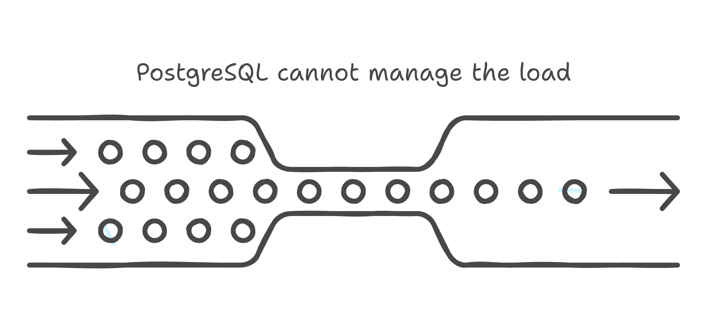
Gotcha 2: Connection pool exhaustion. Airflow's default configuration will happily open more database connections than your PostgreSQL instance can handle. We hit this at 3 AM one morning when 12 parallel extraction tasks each held 4 connections, plus Airflow's own metadata database connections. The fix was a combination of connection pooling with PgBouncer and careful Airflow pool configuration.

Gotcha 3: Sensor deadlocks. We used Airflow sensors to wait for source files to arrive before starting extraction. But sensors occupy a worker slot while waiting. If all your worker slots are occupied by sensors waiting for files that have not arrived, no actual work gets done. We switched to mode="reschedule" for all sensors, which releases the worker slot between pokes.

When an analyst runs a query against 6TB of data, "please wait" is not an acceptable answer. Here are the optimizations that made the biggest difference.

Materialized Views for Common Aggregations

Risk analysts had a set of 15-20 queries they ran daily. Rather than hitting the fact tables each time, we pre-computed the results:

CREATE MATERIALIZED VIEW mv_institution_risk_summary AS
SELECT
    i.institution_name,
    date_trunc('month', f.event_date) AS month,
    f.event_type,
    COUNT(*) AS event_count,
    SUM(f.amount) AS total_amount,
    AVG(f.amount) AS avg_amount,
    PERCENTILE_CONT(0.95) WITHIN GROUP (ORDER BY f.amount) AS p95_amount
FROM fact_credit_events f
JOIN dim_institution i ON f.institution_key = i.institution_key
WHERE f.event_date >= CURRENT_DATE - INTERVAL '24 months'
GROUP BY 1, 2, 3;

Materialized view refreshes were scheduled as the final step in the daily ETL. A query that took 45 seconds against the raw fact table returned in under 200 milliseconds from the materialized view.

Index Strategy

We followed a principle I call query-driven indexing: no index exists without a documented query that needs it. Every index has a maintenance cost (slower writes, more storage, vacuum overhead), so each one must justify its existence.

The most impactful indices were partial indices:

-- Only index recent, active events (not 7 years of history)
CREATE INDEX idx_recent_active_events
    ON fact_credit_events (borrower_key, event_type)
    WHERE event_date >= '2024-01-01' AND status = 'ACTIVE';

Partial indices gave us the read performance of a full index at a fraction of the storage cost.

Vacuum and Maintenance

PostgreSQL's MVCC architecture means that updates and deletes create dead tuples that need to be cleaned up. At our scale, autovacuum's default settings were woefully insufficient.

We tuned per-table autovacuum settings for our most heavily updated tables:

ALTER TABLE fact_credit_events SET (
    autovacuum_vacuum_threshold = 10000,
    autovacuum_vacuum_scale_factor = 0.01,
    autovacuum_analyze_threshold = 5000,
    autovacuum_analyze_scale_factor = 0.005
);

The default scale factor of 0.2 meant that a table with 500 million rows would not trigger a vacuum until 100 million dead tuples accumulated. That is a recipe for table bloat and degraded performance.

If I were starting this project today, here is what I would do differently:

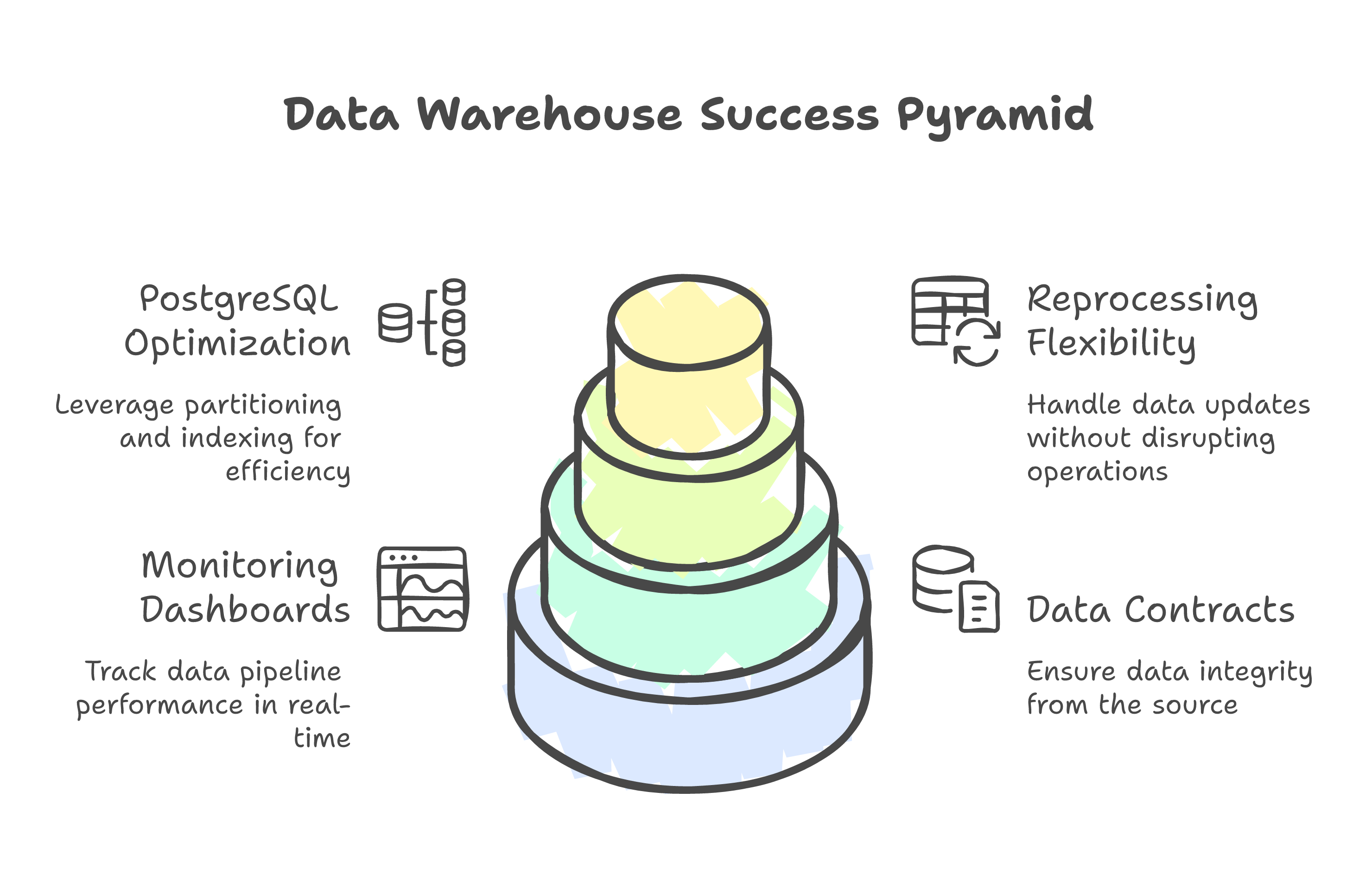
1. Invest in a data contract system from day one. Half our ETL bugs came from upstream schema changes that we discovered at runtime. A formal data contract with schema versioning would have saved dozens of late-night debugging sessions.

2. Build the monitoring dashboard before the pipeline. You need to see what is happening before you can fix what is broken. We built monitoring as an afterthought and paid for it.

3. Plan for re-processing. At some point, you will discover a bug that corrupted three months of data. You need the ability to reprocess any time range without affecting current operations. Design for this from the start.

4. Respect PostgreSQL's strengths. We considered migrating to a columnar database twice. Both times, proper partitioning, indexing, and materialized views got us the performance we needed. PostgreSQL can handle more than most people give it credit for.

Data engineering is not about the tools -- it is about the discipline. The tools will change, but the principles of idempotency, observability, and defensive design will carry you through any scale.

For anyone embarking on a similar journey, feel free to reach out. I am always happy to discuss the war stories that do not make it into documentation.